Landslide Exercise
Landslide Susceptibility Model
Objectives:
Overview
This case study has been chosen to demonstrate the concepts being highlighted by the bootcamp. We have chosen a landslide susceptibility analysis due to the diversity of inputs and a general curiousity into the methodology. The study area has been chosen in response to the Oso Mudslide[^1] which took place in Washington State on March 22nd, 2014. The methodology for this analysis is based off of work done by the California Geological Survey in Conjunction with the USGS[^2].
Datasets
Using the iRODS plugin, download the following layers:
- USA_states.shp
- DEM.tif
- WA_geology.shp
Data Wrangling
Set project projection
Before starting any project in a GIS program, you should first set the project projection to make sure your data comes in with the same extent. If you don't set the project's projection, the program will use the projection of the first layer added or EPSG:4326.
You can set the projection with the following steps:
- In the top navbar go Project > Project Properties
The following window should open up.
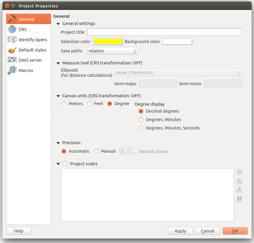
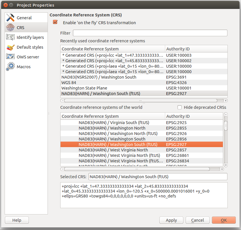
- Select CRS in the Left menu
- Check Enable On-the-fly CRS transformation
- Select NAD83(HARN)/Washington South(ftUS) EPSG:2927 from the List of Projections
Add the US States shapefile
Since our project is directed at the state of Washington, we should use the state boundary as our study area. The Global Administrative Areas[^7] project provides high-quality boundary data on country,state and county levels. We can use the US-state level dataset to get the Washington boundary.
- Open the iRods Plugin and navigate to the Exercise_3 directory
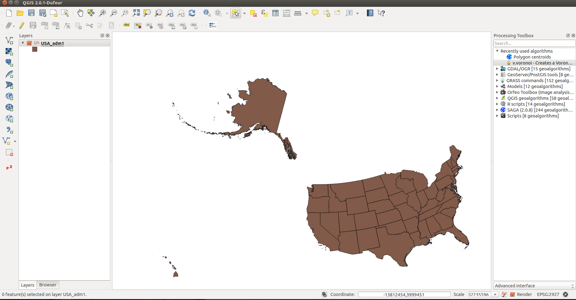
- Load the USA_states.shp layer
Create a layer for the state of Washington
SCreating a layer for the state of Washington will let us define the boundary for our study.
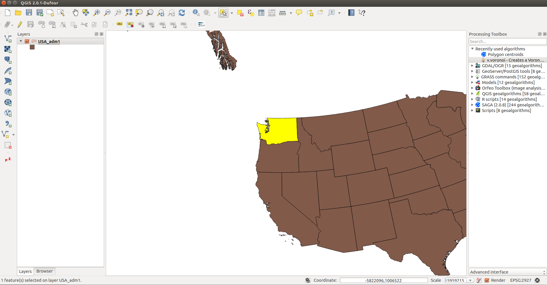
- In the top toolbar, select Select Single Feature
- Click on the state of Washington to select it
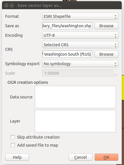
- Right click on the USA_states layer and select Save Selection As...
- Format: ESRI Shapefile
- Save as: washington.shp
- Encoding: UTF-8
- CRS: Project CRS
Load the new washington layer
- Select Add Vector Layer
- Browse to the new washington layer and click *Open*
Remove the USA_states layer from the project
Now that we have the Washington layer, we can get rid of the U.S. layer.
- Right click the layer in the table of contents
- Select Remove
Add the DEM layer from the iPlant data store
DEMs or Digital Elevation Models are very useful for establishing topological context in a map. DEMs generally come as a raster dataset that consists of elevation values. There are several different byproducts that can be created from DEMs.
This DEM was taken from GTOPO30 satellite data.
- Open the iRods plugin and navigate to the directory Exercise_3
- Select DEM.tif
- Click Load
Project the DEM
The DEM uses the WGS 84 coordinate system, which means it is measured in degrees. Since our project is in Washington State Plane which is measured in meters, we need to reproject the DEM to use it in our analysis.
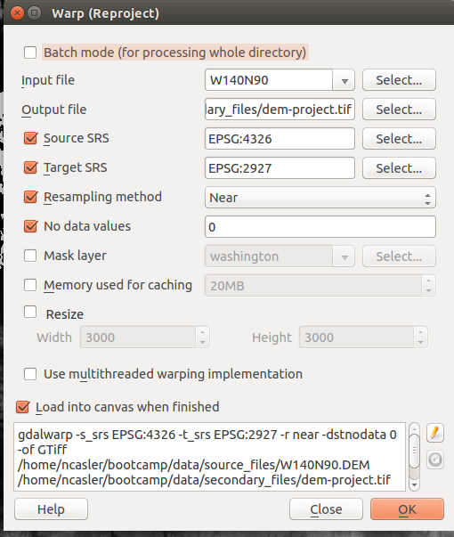
- In the top menu, go to Raster > Projections > Warp (Reproject)
- Use the following options
- Input File: DEM
- Output File: dem_project.tif
- Source SRS: EPSG:4326
- Resampling Method: Near
- No data values: 0
Clip the dem to the state of Washington
Clipping the dem will remove any values outside of the study area, which will make the analysis more efficient.
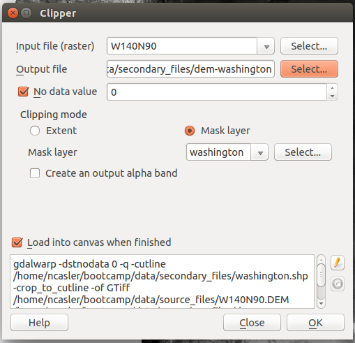
- In the top menu, select Raster > Extraction > Clipper
- In the window, set the following options:
- Input file: dem_project.tif
- Output file: WA_dem.tif
- No data value: 0
- Clipping Mode: Mask layer > washington
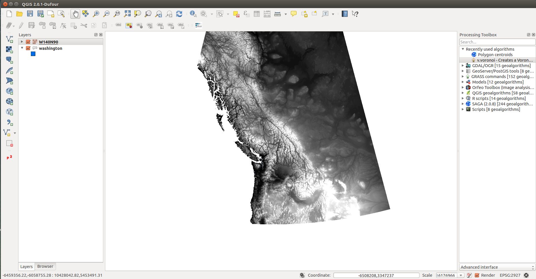
- Load into canvas when finished
- Remove the DEM layer
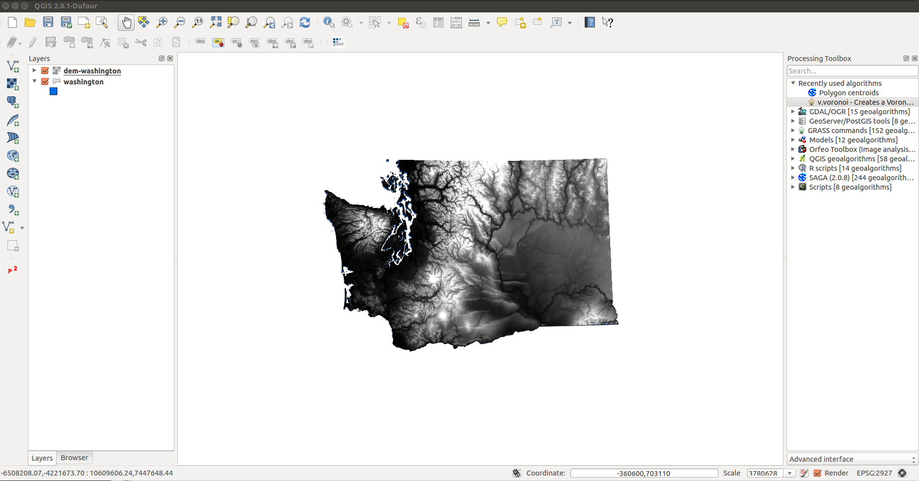
The project area should now look like this:
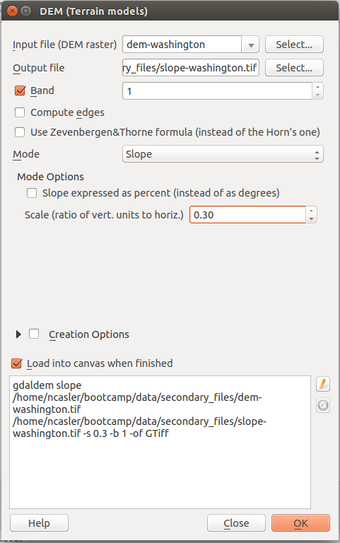
Create a slope surface
- In the top menu, select Raster > Analysis > DEM
- Input file: WA_dem
- Output file: WA_slope.tif
- Mode: Slope
- Scale: 0.30
- Load into canvas when finished
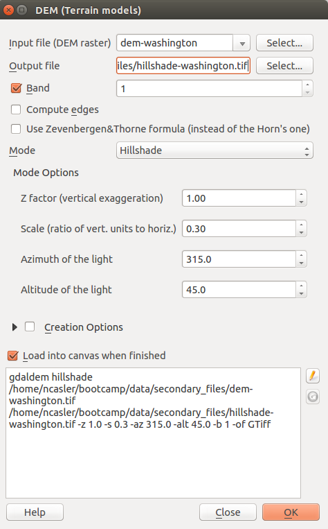
Create a hillshade layer
- In the top menu, select Raster > Analysis > DEM
- Input file: WA_dem
- Output file: WA_hillshade.tif
- Mode: Hillshade
- Z factor: 1.0
- Scale: 0.30
- Azimuth of light: 315.0
- Altitude of light: 45.0
- Load into canvas when finished
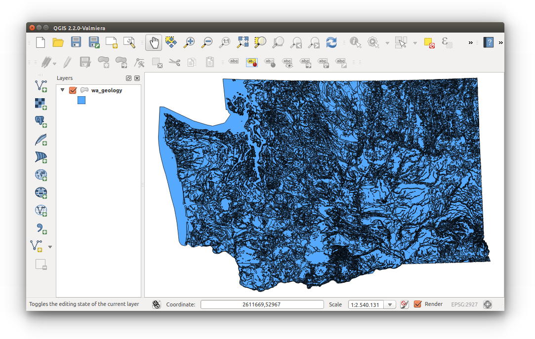
Load the Geology Layer
- Open the iRods plugin
- Load the WA_geology.shp file
Add Rock strength index
We are going to create a numeric field to represent the strength of the geologic unit
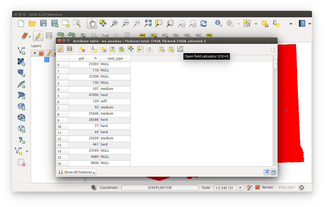
- Open field calculator in Attribute Table:
- Right-click WA_geology in Layers List > Open Attribute Table > Toggle editing mode (top left)
- While in edit mode,click Open field calculator (top right)
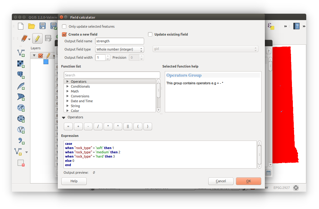
- Add and calculate new field
Match your Field Calculator window to the one below for creating a new field strength with a range of values of 0-3. Be sure to match it exactly as it's displayed
Note: double-quotes are evaluated as a column whereas single-quotes are evaluated as column values. Save your changes once finished.
Expression:
      case

          when "rock_type" = 'soft' then 1

          when "rock_type" = 'medium' then 2

          when "rock_type" = 'hard' then 3

      else 0

      done
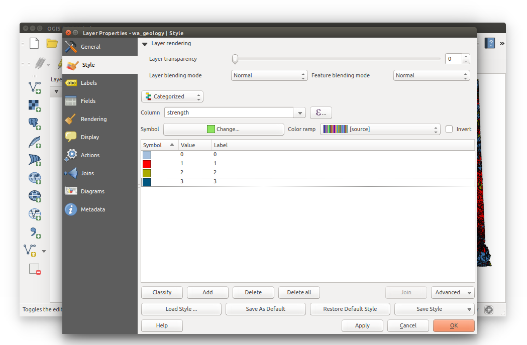
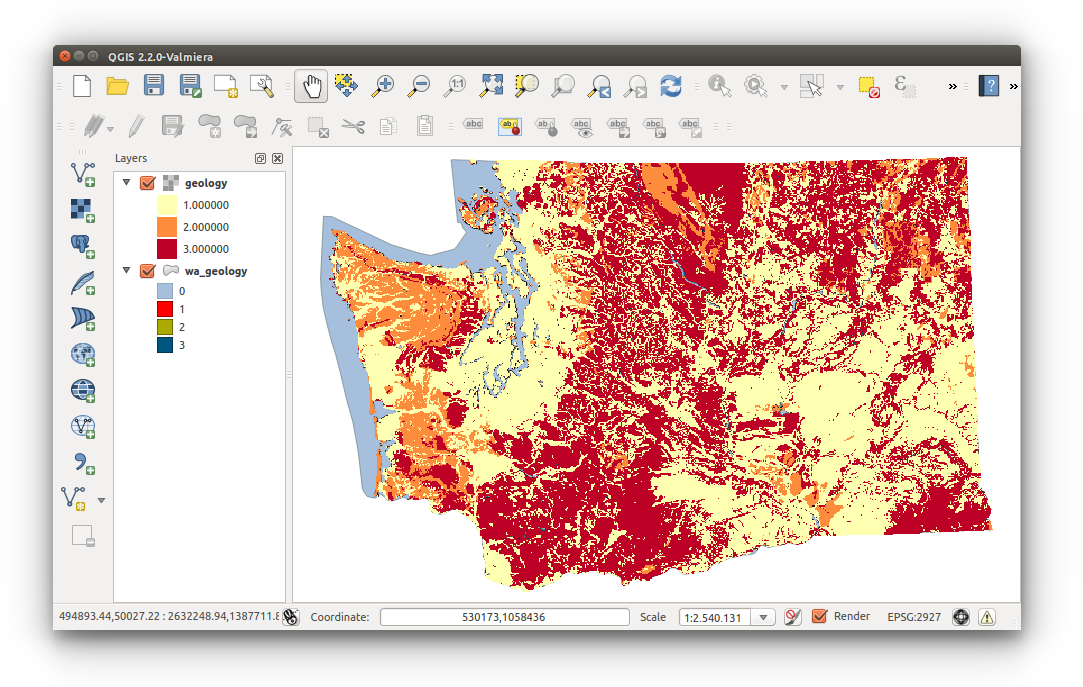
Visualize the geology by strength
- Right-click on WA_geology.shp in Layer List > Properties > Style
- Change style type from Single Symbol to Categorized.
- Categorize by strength and click Classify to add classes.
- Match your colors with the example below or get fancy with your own styling.
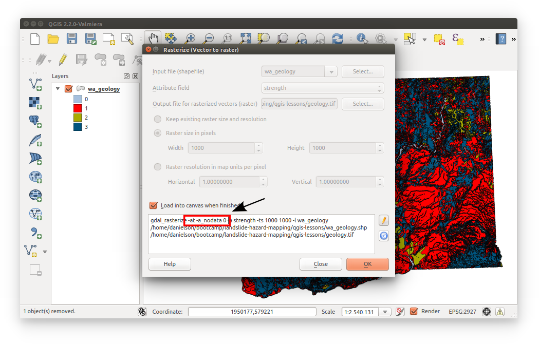
Rasterize the rock strength layer
GDAL's rasterize is a prefered method. This can be accessed through Menu Bar > Raster > Conversion > Rasterize (Vector to raster). Notice how the parameters have been diabled in the example below. There's a specific reason for this. Complete the parameter inputs: Define your output file and location (in working directory); Attribute field = strength; Raster size in pixels = 1000 x 1000. Because GDAL is more powerful in the commandline, there are certain parameters that cannot be set within QGIS.
- Click the edit icon (pencil) locate near the block of code. This enables you to add custom parameters.
- Add the line of code
-at -a_nodata 0just aftergdal_rasterize
The-atflag enables the ALL_TOUCHED rasterization option so that all pixels touched by lines or polygons will be updated, not just those on the line render path, or whose center point is within the polygon. Defaults to disabled for normal rendering rules.[^3] -a_nodata 0The above snippet specifies that 0 should be recognized as a missing or null value, which prevents pixels with 0 value from being visualized or used in analysis in the output raster.[^3]
Style the new Rock Strength Raster
- Open WA_geology.tif style properties. HINT: See step 4.
- For Render type, select Singleband pseudocolor
- On the right select:
- Load min/max values: Min/max;
- Extend: Actual (slower); then Load.
- Change Mode to Equal Interval with 3 classes. Remember, we only have three rock strength classes: soft, medium, hard. Change your color map if you'd like. The color maps are not stored into the raster, so the raster will load with the default color map (black to white) each time its opened in a new project.
- Click Classify. Apply and OK.
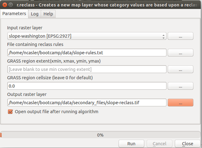
- Input Raster: WA_slope
- File containing reclass rules: slope-rules.txt
- Output raster layer: slope-reclass.tif (NOTE: select Save to file... or else QGIS will not create a permanent output)
Data Analysis
Reclassifying inputs:
Slope
Category Slope 1 < 3° 2 3-5° 3 5-10° 4 10-15° 5 15-20° 6 20-30° 7 30-40° 8 > 40° In order to reclass our slope layer into something useful, we will use the grass r.reclass tool
The r.reclass tool reads text files which define the classification rules(rule files). For this example, our rule fill will have the following contents:
slope-rule.txt
0 thru 2.99 = 1

3 thru 4.99 = 2

5 thru 9.99 = 3

10 thru 14.99 = 4

15 thru 19.99 = 5

20 thru 29.99 = 6

30 thru 39.99 = 7

40 thru 90 = 8
Once we have created the slope rule file. We can select the r.reclass tool from the Processing Toolbox.
In the processing toolbox, select GRASS commands > Raster > r.reclass
We will use the following settings for the reclassify tool:
Susceptibility
We will have to do some raster calculations to create the output data set. The classifications are taken from the California study[^2] and are as follows:
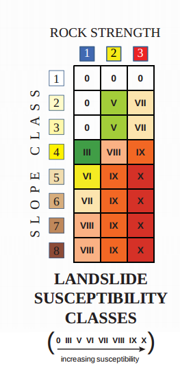
Since we need to cross reference these categories, we need to create a raster which represents each unique combination of the slope and rock strength classes. A method to create unique combinations is to promote the rock strength categories a decimal place. This would make the rock classes: 10,20, and 30.
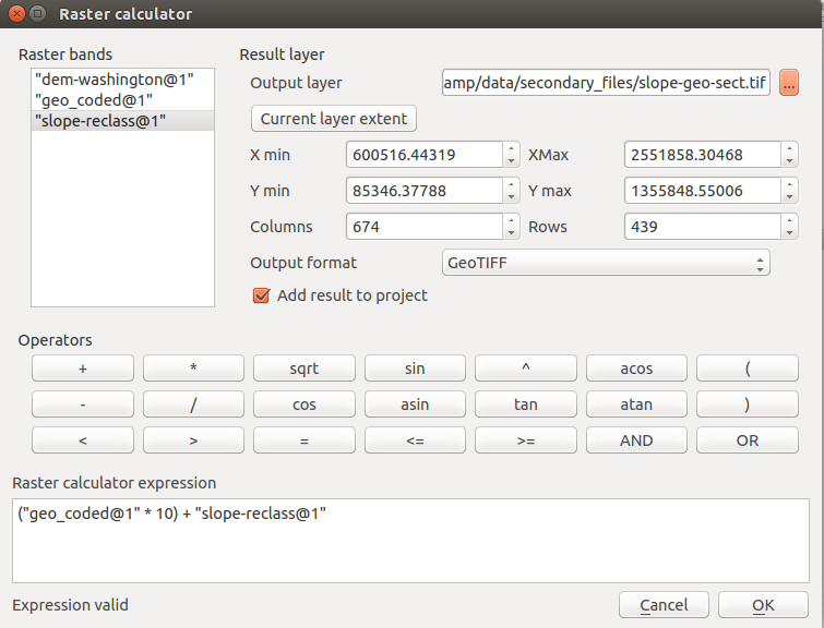
To create these new classes, we can load the WA_geology.tif, and slope-reclass.tif
In the top menu, select Raster > Raster Calculator
Our raster calculator expression will be:
("geo_coded@1" * 10) + "slope-reclass@1"Output layer: slope-geo-sect.tif
We can apply the landslide susceptibility classification using r.reclass and the following rule file:
landslide-rule.txt
11 12 13 21 31 = 0

14 = 3

22 23 = 5

15 = 6

16 32 33 = 7

17 18 24 = 8

25 thru 28 34 = 9

35 thru 38 = 10
Continue to SHOW YOUR RESULTS
[^1]: http://www.usgs.gov/blogs/features/usgs_top_story/landslide-in-washington-state [^2]: http://www.conservation.ca.gov/cgs/information/publications/Documents/MS58.pdf [^3]: http://www.spatialreference.org/ref/epsg/2927 [^4]: https://lta.cr.usgs.goc/GTOPO30 [^5]: http://www.dnr.wa.gov/ResearchScience/Topics/GeosciencesData/Pages/gis_data.aspx [^6]: http://wdfw.wa.gov/conservation/gap/land_cover_data.html [^7]: http://www.esrl.noaa.gov/thredds/catalog/Datasets/cpc_us_precip/catalog.xml#Datasets/cpc_us_precip/RT [^8]: http://gadm.org/country