Pre-requisites: Intro to Spatial Data, Data Formatting

Objectives:

• Recognize a few spatial relationships
• Understand how to clip a raster

Spatial Functions

Relational Operations

Relational operators are a set of methods used to test for the existence of a specified toplogical spatial relationship between two geometric objects as they would be represented on a map. The basic approach to comparing towo geometric objects is to project the objects onto the 2D horizonal coordinate reference system representing the Earth’s surface, and then make pair-wise test of the intersections between the interiors, boundaries and exteriors of the twp projections and to classify the map relationship between the two geometric objects based on the entries in the resulting 3 by 3 intersection matrix.¹

	b
a	Interior Boundary Exterior Interior   dim[{{{1}}}] = 2     dim[{{{1}}}] = 1     dim[{{{1}}}] = 2   Boundary   dim[{{{1}}}] = 1     dim[{{{1}}}] = 0     dim[{{{1}}}] = 1   Exterior   dim[{{{1}}}] = 2     dim[{{{1}}}] = 1     dim[{{{1}}}] = 2

Spatial Predicates

The above figure demonstrates the criteria outlined by the Dimensionally Extended Nine-Intersection Model(DE-9IM). The matrix is used to outline specific spatial relationships or predicates which are more accessible to interpretaion. These named spatial predicates are also used by spatial queryies to selet subsets of geometrys that fit in one spatial predicate.

Here is a quick outline of the Spatial Predicates

Equals

The two geometric objects are spatially equal meaning, they represent the same geometry (congruent in geometric terms)

Disjoint

The two geometric objects share no points in common, the two objects are completely separate

Intersects

The two geometric objects have at least one point in common

Touches

The two geometric objects have at least one boundary point in common, but no interior points

Crosses

The two geometric objects share some but not all interior points

Contains

One geometry is contained by the other if all the points of one geometry are within the boundary or interior of the other and they share at least one interior point. This means that this predicate may produce unpredictable behavior for linestrings and points which have no interior points.²

Within

The inverse of Contains. The first geometry is completely within the second geometry

Overlaps

The two geometries share some but not all points in common, the two geometries have the same dimensions and the intersection of the two geometries has the same dimension as the two input geometries

Covers

Similar to contains, but does not require that the two geometries share an interior point, which makes it the proper tool for working with inputs of different dimensions.

Methods for Spatial Analysis

There are a few standard methods for geometric analysis available based on the geoetric object model. This is a brief listing of basic analyses and is by no means exhaustive of the available functions.

Distance

Measures the shortest distance between two geometries.

Buffer

Creates a geometric object that represents all points within a given distance from the given geometry

Convex Hull

Creates a geometric object that represent the minimum bounding convex polygon that contains all points of the given geometry

Intersection

Returns a geometric object that represents the intersecting parts of two given geometries

Union

Creates a geometric object that represents the combination of two given geometries

Difference

Returns the given geometries that do not intersect. If all gemetries intersect, an empty set will be returned.

Symmetric Difference

Creates a geometric object of the disjoint parts of two geometries. The output will have all pieceheld by one geometry or the other, but not the areas held by both.

Examples

• Intersection
  • All rivers within washington state boundary
  • Residential areas with past landslide
• Union
  • Merging census data for two states in a single layer (Useful for studying phenomena that do not respect political boundaries)
  • Merging state boundaries for Canada, U.S. and Mexico into a North American dataset (GADM makes this a breeze)
• Buffer
  • Instagram posts vs within 100m of a local restaurant
  • Tweets vs within 1km of a football stadium
• Convex Hull
  • Bounding boxes, circles
  • Range modeling for small data sets

Raster Functions

• Slope - This function will calculate a slope surface given a raster holding an elevation model
• Aspect - This outputs a surface holding values 0-360 referencing the azimuth of the given surface
• Raster Calculator - Performs a designated mathematical equation on all values within a raster. This can also be used to combine/difference rasters.
• Interpolation - Useful for resurfacing a dataset. This can also be used to create a continuous surface from a point dataset.
• Reclassify - Useful for creating discrete value categories from continous values(e.g.float data) also useful for creating presence absence datasets.
• Polygonize - Creates a set of polygon features representing the given raster dataset
• Histogram - Create a histogram showing the distribution of values in a raster dataset

Exercise

The following exercises are a continuation of the previous exercises. Open your project workspace before starting the following steps. See Data Wrangling.

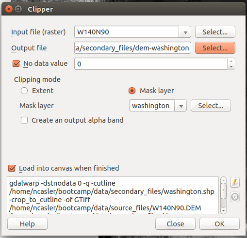
1. Clip the dem to the state boundary
   • In the top menu, select Raster > Extraction > Clipper
   • In the window, set the following options:
   • Input file: dem-project.tif
   • Output file: dem-washington.tif
   • No data value: 0
   • Clipping Mode: Mask layer > washington
   • Load into canvas when finished
     
2. Remove the dem-project.tif layer
   
   
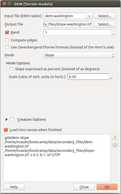
3. Create a slope surface
   In the top menu, select Raster > Analysis > DEM
   
   • Input file: dem-washington
   • Output file: slope-washington.tif
   • Mode: Slope
   • Scale: 0.30
   • Load into canvas when finished
     
     
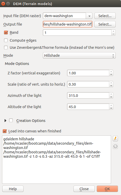
4. Create a hillshade layer
   In the top menu, select Raster > Analysis > DEM
   
   • Input file: dem-washington
   • Output file: hillshade-washington.tif
   • Mode: Hillshade
   • Z factor: 1.0
   • Scale: 0.30
   • Azimuth of light: 315.0
   • Altitude of light: 45.0
   • Load into canvas when finished
     
     
5. Save your project workspace.

• [^3] : Esri
• [^4] : PostGIS Reference Manual. http://postgis.org/documentation/manual-svn/using_postigs_dbmanagement.html