Vector Analysis
Vector Analysis
What this module covers:
- Buffer polylines
- Join census housing (home values) to census tracts (shapefile)
- Intersecting vector layers
Objective:
Quantify total home value at risk within landslide/mass-wasting and fautls.
Data Collection: (there needs to be instructions/quick lesson on each of the collection sources)
- Census housing data - American FactFinder
- Census tracts - TIGER Data
- Quaternary faults - USGS
- Washington seismogenic features - REQUIRES GDAL filegdb driver!
- Washington streams/rivers - USGS National Hydrography Dataset
Here, the data are pre-wrangled (located on nathan’s server, for now):
- faults_100k - [source]
- housing-data.zip
Clean your Data:
Wrangle Census Data:
Luckily, the Census data has already been wrangled. Census data can sometimes be tricky.
High-risk rules:
- within 100m of fault lines
- within 50m of rivers/streams
- within soft geologic areas
- Open QGIS and configure project workspace.
- Import data:
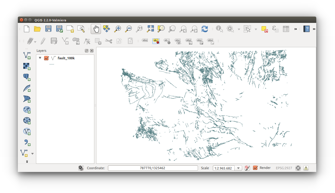
- HINT: The project projection will default to the first layer that is added to the project (See lower right of image below: EPSG:2927).
- Add Vector Layer:

fault_100k.shp
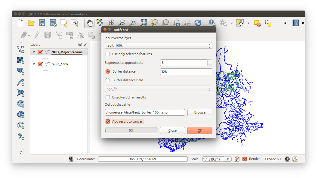
- Buffer fault lines to 100m:
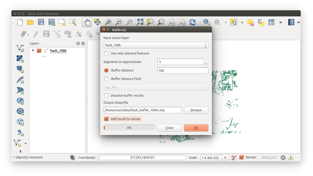
- Menu Bar > Vector > Geoprocessing Tools > Buffer(s)
- Configure inputs as follows:
Input vector layer: fault_100k
Buffer distance: 100
Output shapefile: fault_buffer_100m.shp
Add results to canvas: (Checked)
Click OK to perform analysis, Close to exit the tool
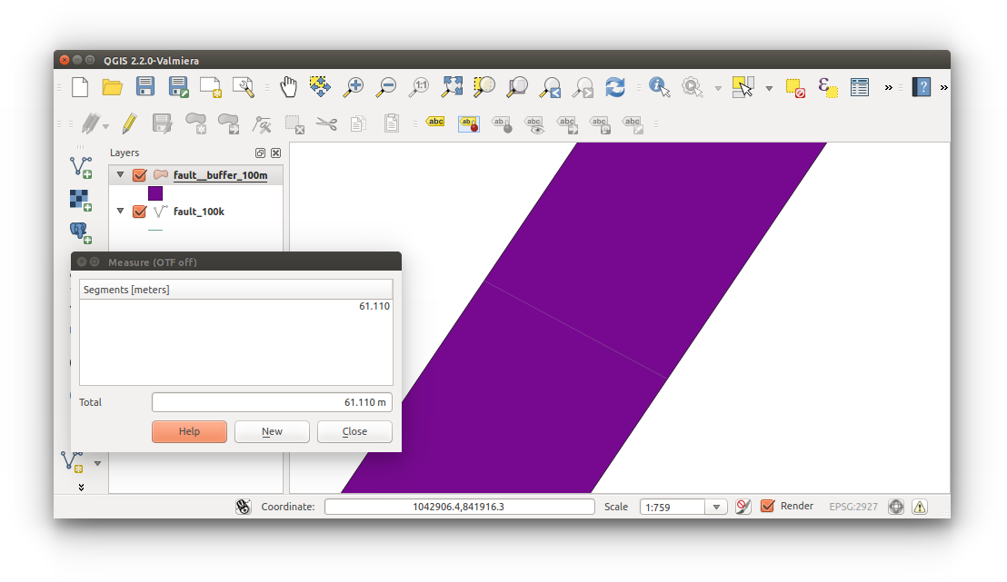
- Zoom in to a buffer, close enough to see the width
- Open the meaure tool

- Measure the width of the buffer. Notice how the total width is only about 62 meters, or 100 feet. Current map units are determined by the CRS, in this case EPSG:2927 is in US feet and we need meters. Simply changing the CRS in Project Properties does not give us the correct results- this is still measured from EPSG:2927 US feet.
Important:
There are two methods to perfoming a buffer analysis on our shapefile. The problem here is that our CRS is EPSG:2927 (in US feet) and the buffer distance is based on map units (still US feet). The two methods are: convert 100 meters to US feet and use this value in the buffer analysis while maintaining EPSG:2927 (in US feet); OR, reproject the layer thus creating a new file with a CRS in meters (correct map units), and then reprojecting back to EPSG:2927. We’ll go with the former.
- Now we need to perform the buffer analysis with the correct method. Remove the incorrect buffer layer: fault_buffer_100m.shp
- Add Vector Layer:
- NHD_MajorStreams.shp
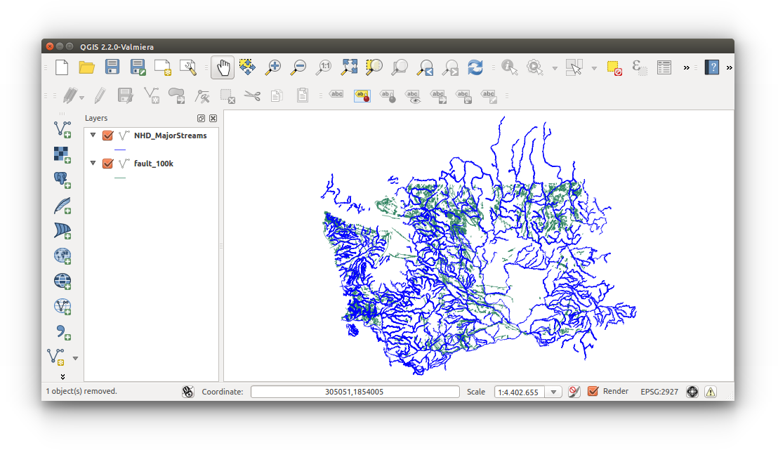
- NHD_MajorStreams.shp
- Open the buffer tool:
- Menu Bar > Vector > Geoprocessing Tools > Buffer(s)
- Buffer fault_100k:
- Configure inputs as follow:
Input vector layer: fault_100k
Buffer distance: 328
Output shapefile: fault_buffer_100m.shp
Add result to canvas: (Checked)
Click OK to run (overwrite necessary), and CLOSE to exit tool
Reminder:
Buffer distance = 100 meters * 3.28084 feet = 328.084 feet
1 meter = 3.28084 feet
- Configure inputs as follow:
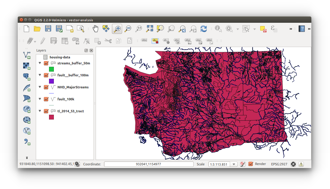
- Confirm 100 meter buffer on faults:
- Open measure tool and confirm 200 meter total width (100 meters * 2 = 200 meters)
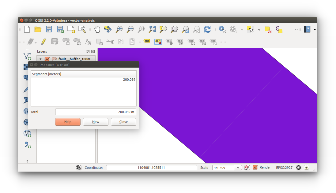
- Open measure tool
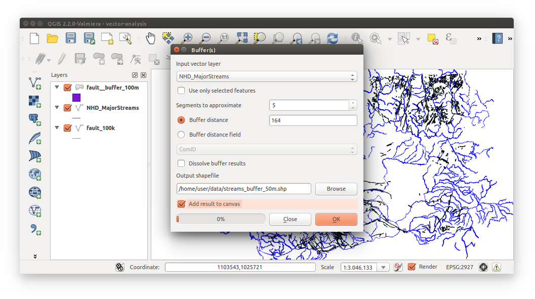
- Repeat buffer with NHD_MajorStreams.shp
- Configure inputs as follows:
Input vector layer: NHD_MajorStreams
Buffer distance: 164
Output shapefile: streams_buffer_50m.shp
Add result to canvas: (Checked)
Click OK to run, CLOSE to exit tool
Reminder:
Buffer distance = 50 meters * 3.28084 feet = 164.052 feet
1 meter = 3.28084 feet
- Configure inputs as follows:
- Confirm 50 meter buffer on streams.
- Import Census housing data (wa-housing-data.csv):
- Notice: housing-data.csv has already been wrangled.
- Add Delimited Text Layer
 or Menu Bar > Layer > Add Delimited Text Layer
 - Configure inputs as follows:
File Name: housing-data.csv
File Format: CSV
First record has field names: (Checked)
No geometry (attribute only table): (Selected)
OK to add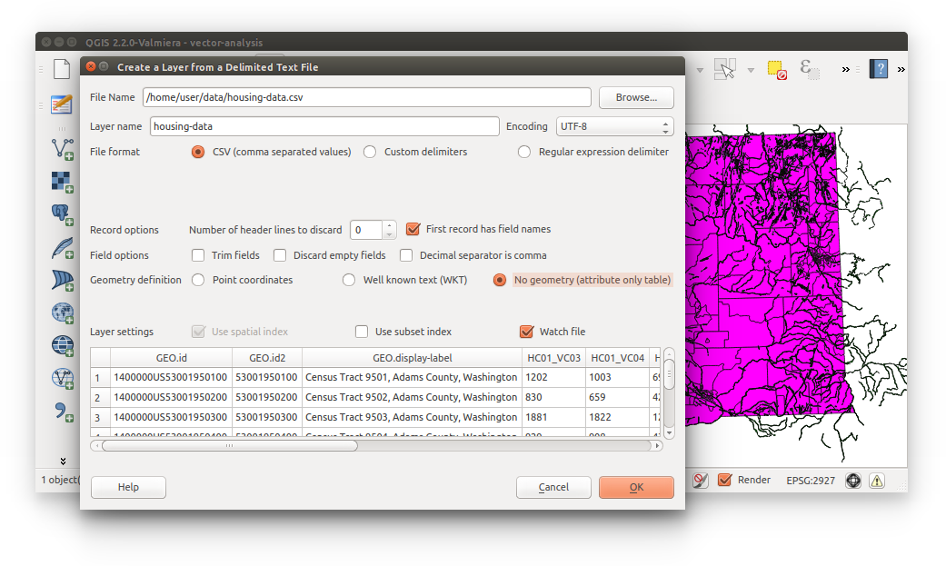
- View Census housing-data.csv:
- Right-click housing-data (in layer list) > Open attribute table
- Import Washington Census tracts (tl_2014__53_tract.shp)
Important: Did you check the projection of the Census tracts shapefile? Be sure your shapefile CRS is EPSG:2927.
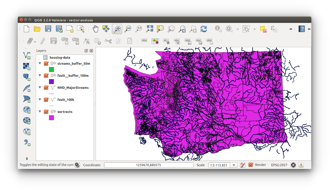
‘on the fly’ projection is selected - Save Census tract (tl_2014_53_tract.shp) with ESPG:2927:
- Right-click tl_2014_53_tract.shp (layer list) > Save As
- Configure as follows: ESRI Shapefile with EPSG:2927, Output filename: wa-tracts.shp, Add saved file to map: (Checked)
- Remove current tl_2014_53_tract.shp
- Open wa-tracts attribute table and housing-data to find the key that will be used to join the tables. HINT: It’s GEOID and GEO.id2.
notes: discuss field types, e.g. cannot compare a string to a number. – add image – - Join Census housing data (housing-data.csv) to Census tracts (wa-tracts.sho):
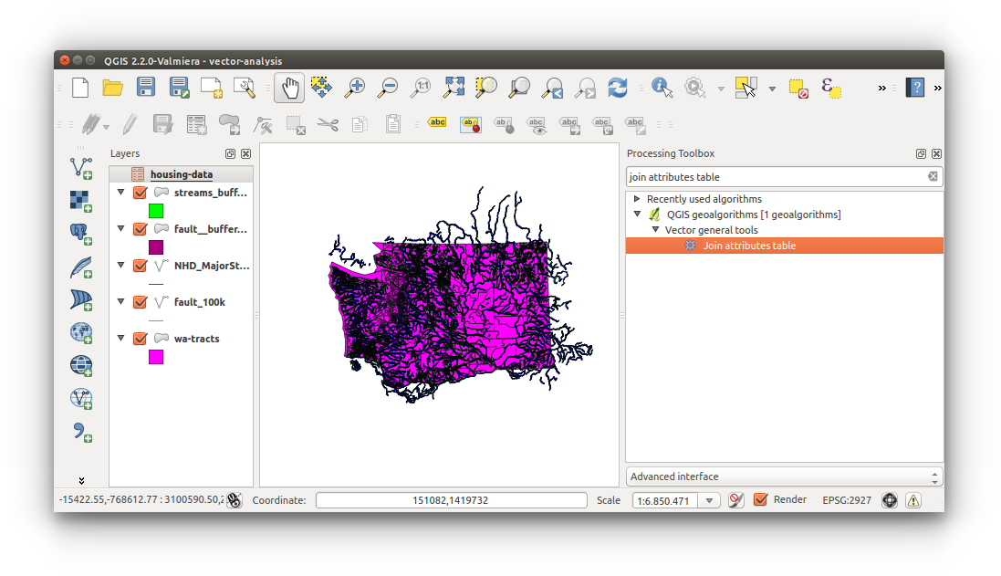
- Open Processing Toolbox (Menu Bar > Processing > Toolbox), search for “join attributes table”, then double-click “Join attributes table”
- Configure Join attributes table as follows:
Input layer: wa-tracts
Input layer 2: housing-data
Table field: GEOID
Table field 2: GEO.id2
Output layer: (Save to file..) tracts-housing-data.shp
IMPORTANT: The concept behind this join is tabular (non-locational-data) joined to spatial data, not spatial data to tabular data. So, you must have spatial data (wa-tracts.shp) as the primary input and tabular data (housing-data.csv) as the secondary input. Notice in the Joing attributes table inputs below.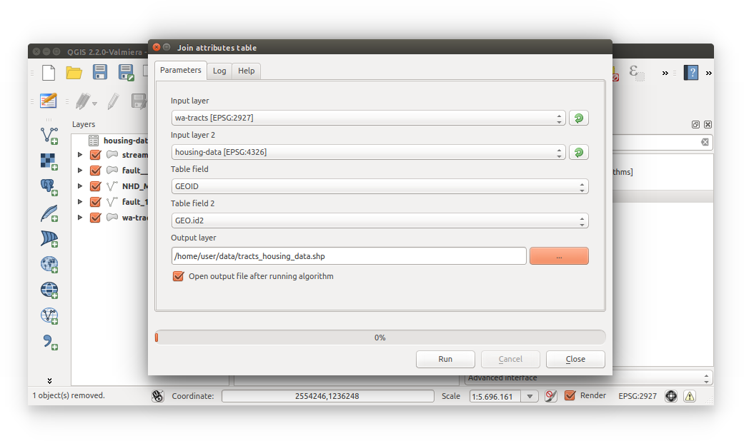
NOTICE: “Layers do not all use the same CRS. This can cause unexpencted results.” Remember, the housing-data.csv does not have any locational data associated with it. Click Yes, to continue.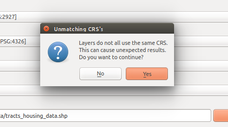
- Open Processing Toolbox (Menu Bar > Processing > Toolbox), search for “join attributes table”, then double-click “Join attributes table”
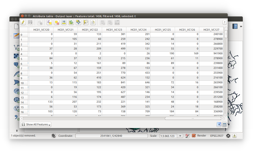
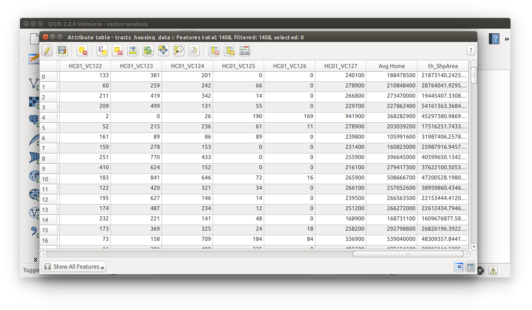
- Confirm output: housing data joined to tracts. Output is named “Output layer”, rename to “tracts_housing_data.shp” (right-click layer > Rename). Hover over the layer in the layer list to view the source path.
- Normalize housing data - tract house count X median tract house value = total tract home value: (you’ll need point data to have a more accurate analysis)
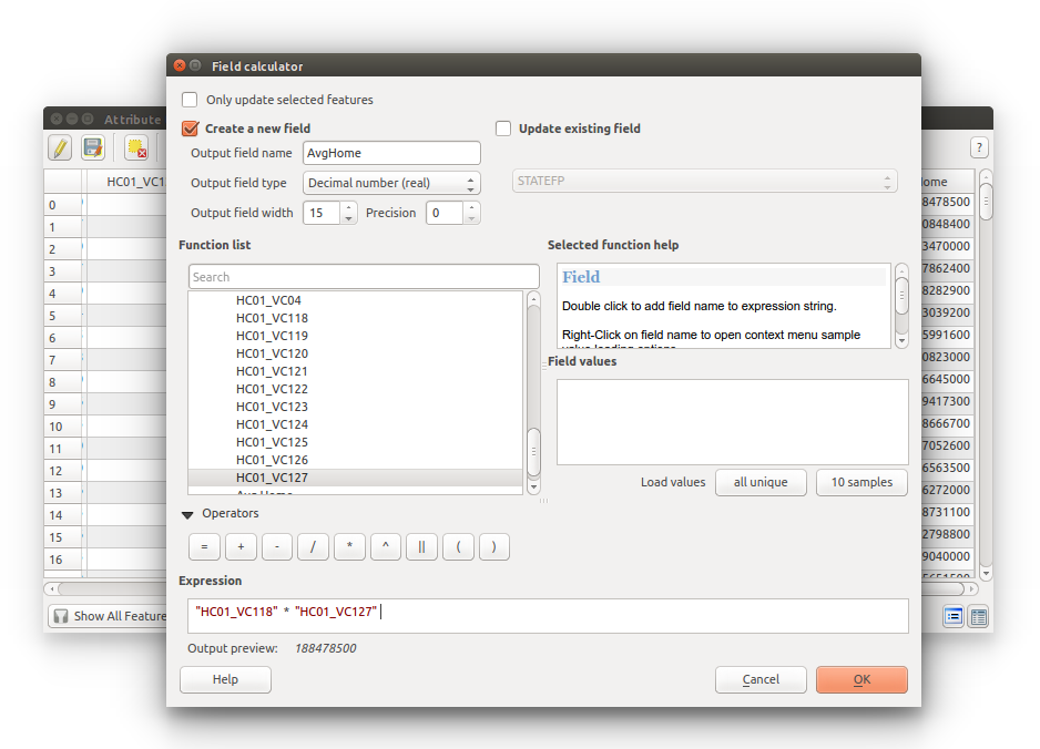
- Right-click tracts_housing_data > Open Attribute Table > Toggle editing mode > Open field calculator
- If you had downloaded the original ACS .csv with annotations then you would be able to easily find what the column headers mean. Or, you could locate the ACS metadata. But we have provided the difinitions below:
HC01_VC118 = Total Housing Units (Owner-occupied)
HC01_VC127 = Estimated Median Housing Unit (Owner-occupied)
We would have calculated total housing * median housing (total) but the ACS does not provide these metrics. - Configure inputs as follows:
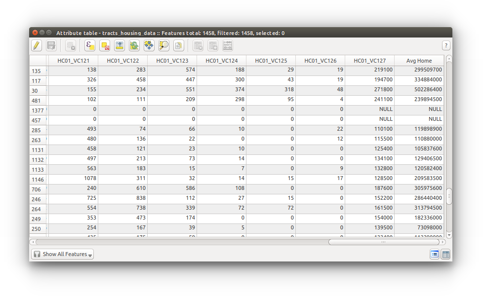
- View your ouputs. Notice there are some NULL values:
- intersect buffered-merged-joined data with reclassified-rasterized geology layer
- intersect buffered faults and streams:
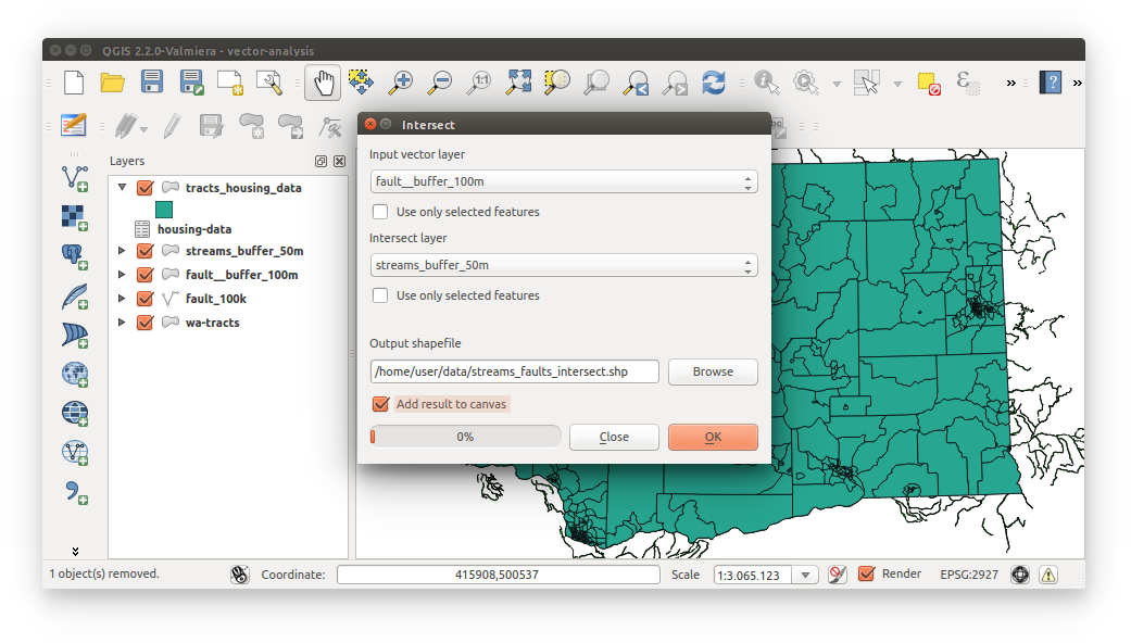
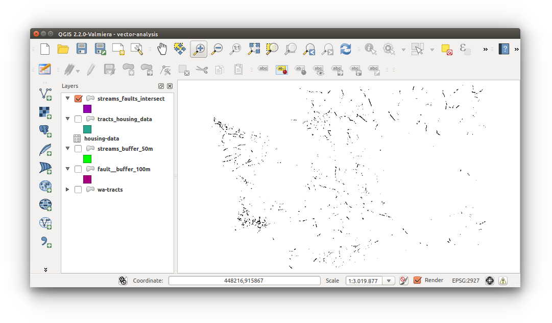
- intersect buffered faults and streams:
- calculate stream_fault_intersection shape area:
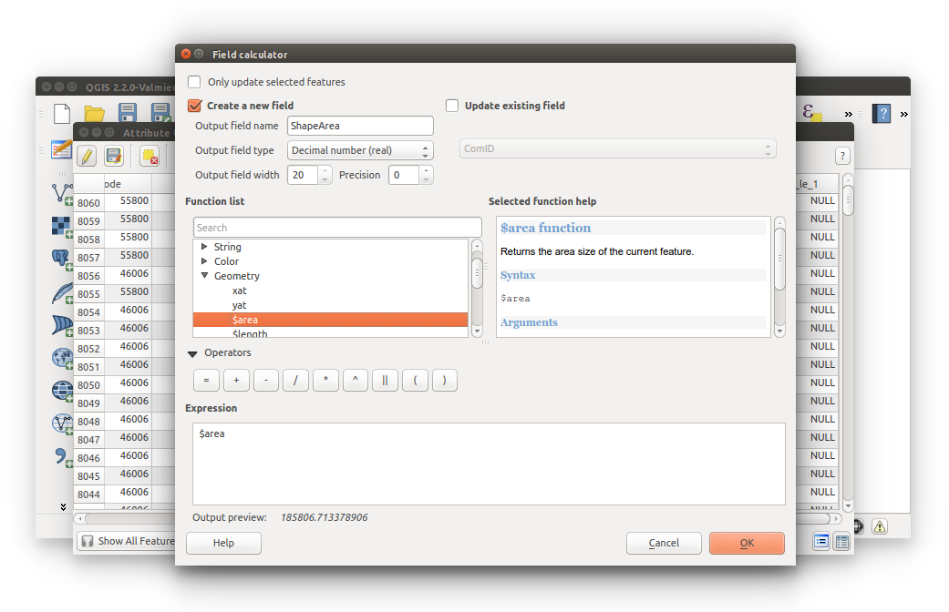
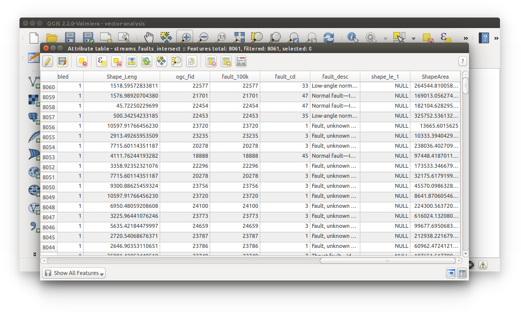
- calculate tracts_housing shape area:
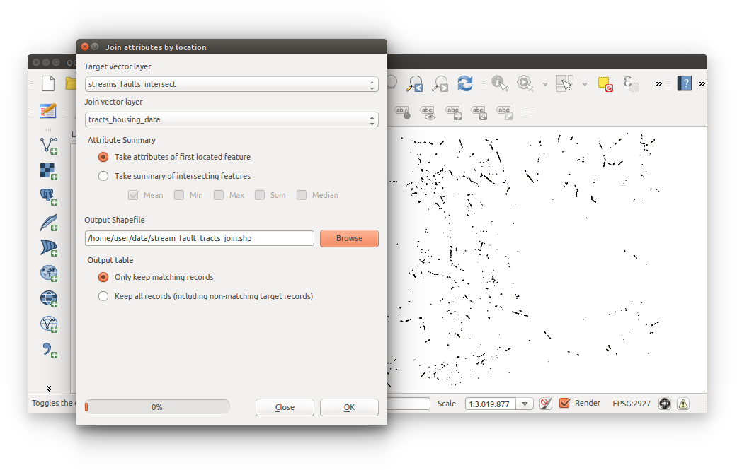
- spatial join stream_fault_intersection + tracts_housing: (this one takes a while)
- data will be used in Raster Analysis