Species Range Modeling with Maxent

Scope

This lesson will take us through the steps involved in creating a species range model using the Maximum Entropy probability distribution.

Before we load in any data we should set the project projection.

To add this to QGIS you can go into the top menu:

Settings > Custom CRS…

Click Add new CRS to create a new custom projection

In the box labeled Name: enter New World LAEA

Under parameters enter the following Proj4 string:

+proj=laea +lat_0=15 +lon_0=-80 +x_0=0 +y_0=0 +ellps=WGS84 +toWGS84=0,0,0,0,0,0,0 +units=m +no_defs

The window should look like this:

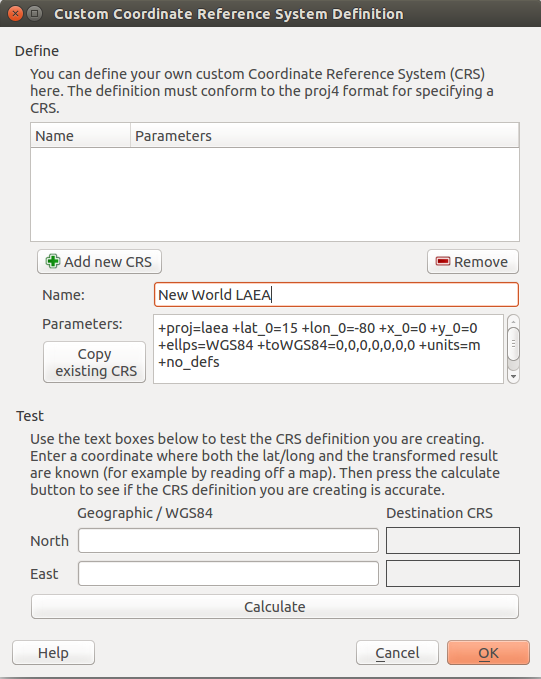
Click OK to exit the window

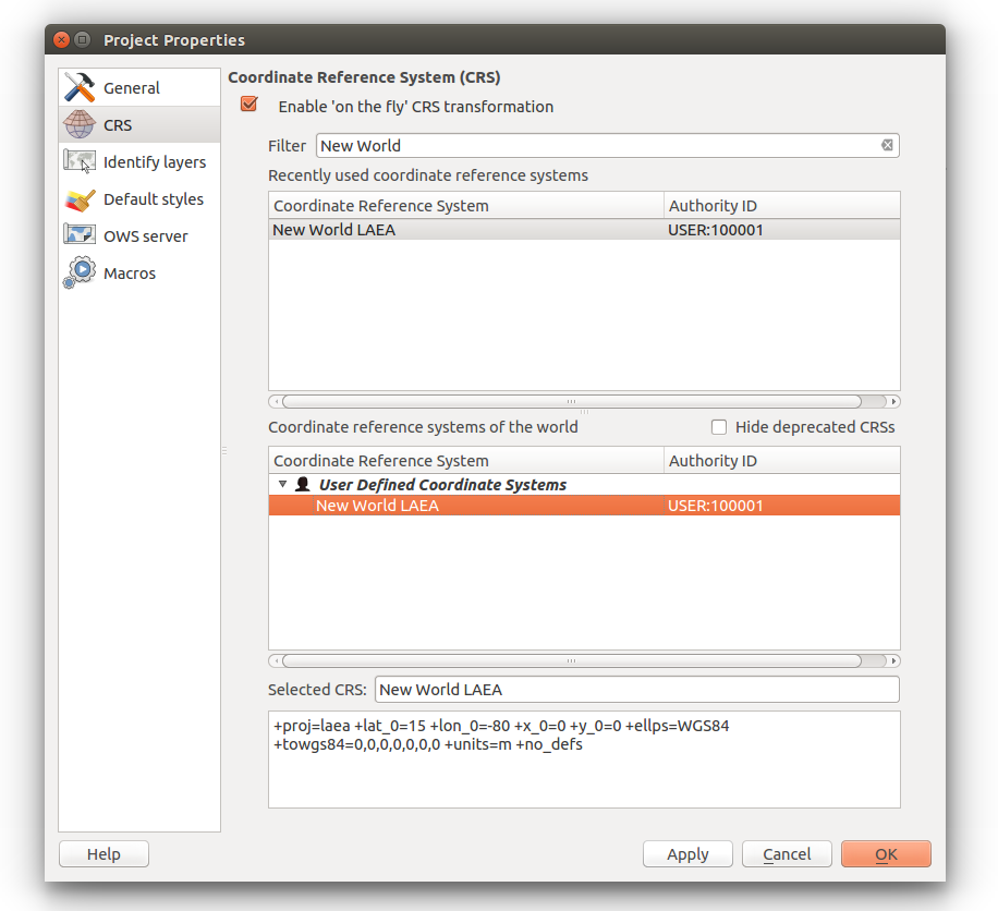
To make set the project projection, in the top menu select Project > Project Properies

You will need to select Enable ‘on the fly’ CRS transformation to set the projection.

You can either scroll through the choices in the second window, or filter them by the string “New World”

Select the projection in the second window and Click Apply

Data Collection

This model will require a comma-separated list of species observation locations.

There are two viable inputs to the modeling algorithm:

CSV with species name, longitude, latitude

SWD file with raster values sampled from points

Since the SWD files make the Maximum entropy algorithm much more performant, we will create one from a regular csv.

We can use QGIS to create these files.

The workflow is as follows:

Load a species shapefile:

We will be loading the layers for this exercise using the QGIS Irods plugin.

iRods

To install the plugin, in the Top Menu go to Plugins > Manage and Install Plugins…

In the left sidebar click Get more

You can either scroll through the plugins or search for iRods

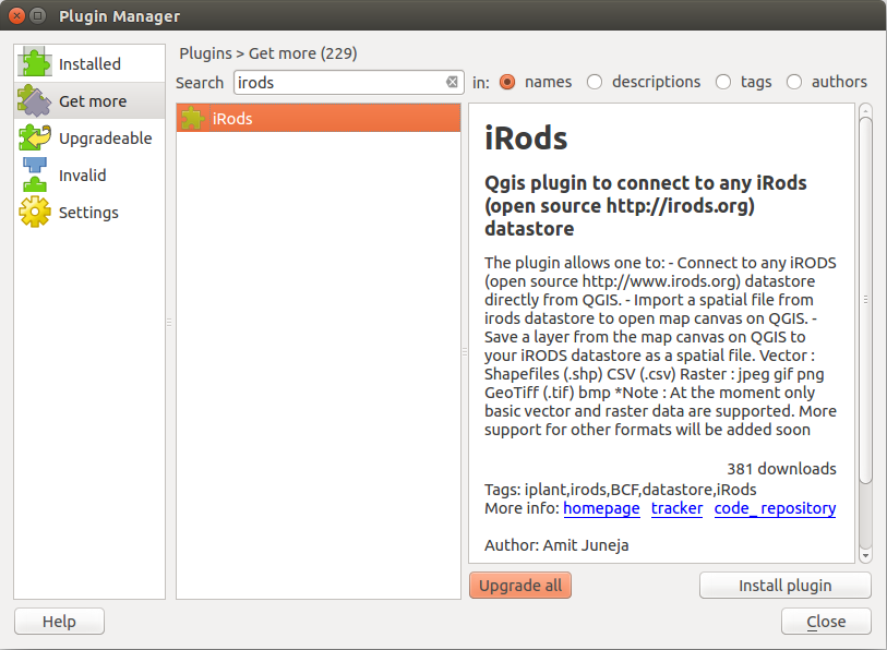
You can install the plugin by clicking Install plugin and you should receive this message

You can now click on Installed in the left sidebar to ensure that the iRods plugin is both installed and enabled.

If you have already set up your iPlant account and were given permissions to the Bootcamp dataset continue to the next steps.

If not, make sure to register for iPlant access, and request access to the data store.

Once, you have access to the data store you can open up the iRods plugin to view the available datasets.

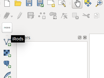
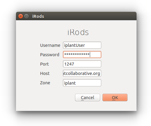
Once you click on the iRods icon, a window should show up where you can enter in your iplant account credentials

This should open up a window with your local files, to get to the Bootcamp files, you will have to set the directory using Set Datastore

In the bottom right of the window click Set Datastore

In the next prompt, enter “/iplant/home/shared/aegis/Spatial-bootcamp”

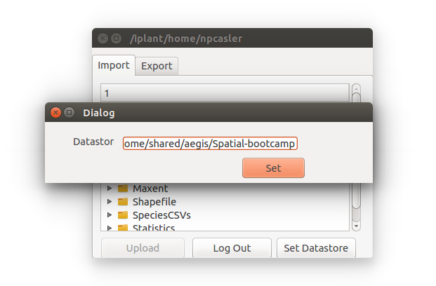
Click set to close the dialog.

You should see a new window with a series of directories.

For this exercise our files will be found under “Range-model”

We can use the Abies amabilis shapefile titled: Abies_amabilis.shp

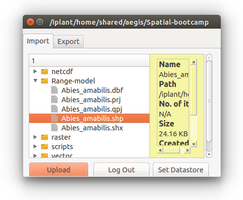
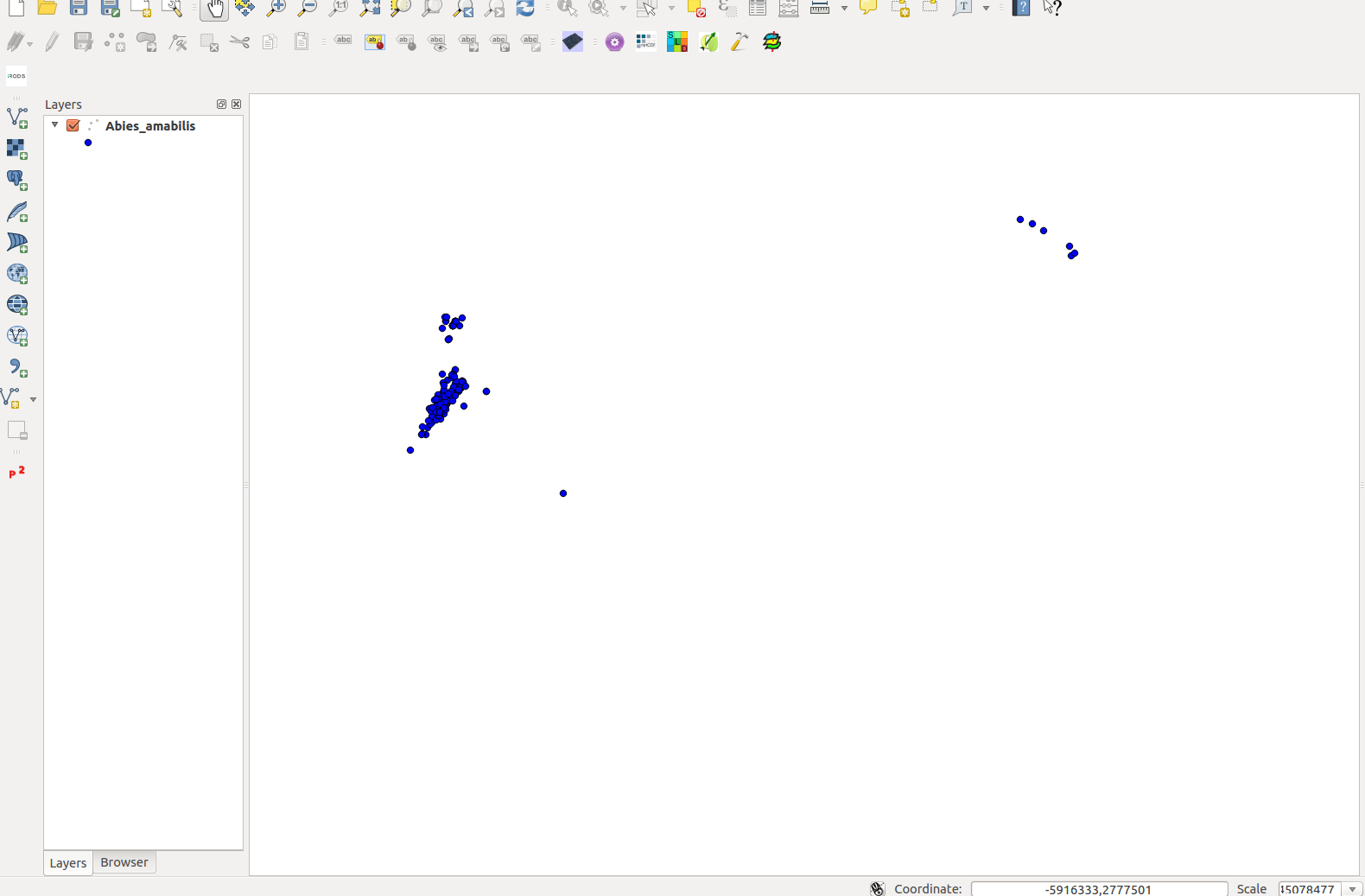
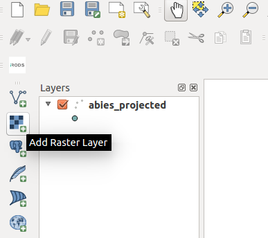
The layer name should come up in the left Table of Contents and the points should show up on the center panel.

Since the Species CSV comes in EPSG:4326, and the environmental variables come in a custom projection, we will need to repojrect the species layer.

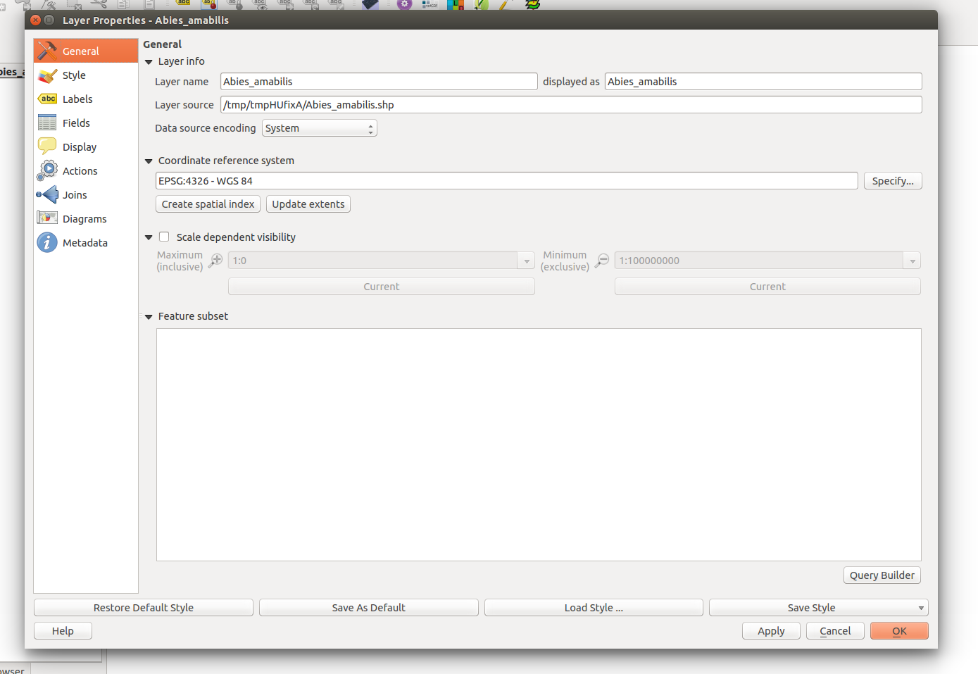
To check the species projection you can right-click the Abies_amabilis in the Table of Contents and select Properties

The Layer properties window will display the layer’s Coordinate Reference System:

To change the projection, you can close out of the Layer Properties window.

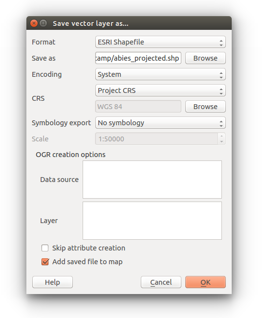
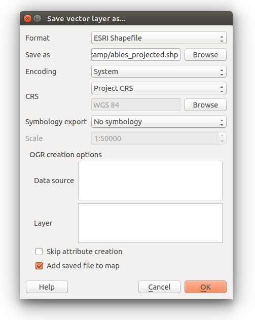
Right click the Abies_amabilis layer in the Table of Contents and select Save as…

You can leave the format as ESRI Shapefile

Click browse to set the location for the output file and name it abies_projected.

Under CRS select Project CRS

Finally check the Add saved file to map option

Right click the new layer and check the layer Properties to make sure the Coordinate Reference System is New World LAEA

If the projection matches, you can remove the original Abies_amabilis layer from the Table of Contents by Right-clicking and selecting Remove

Now that you have the points projected. We need to import the environmental layers.

These files will be stored in the sub-directory Range-model/env

They will need to be downloaded however, so the gdal drivers can merge them.

The environmental layers can be found in the iPlant data store in the env.zip file.

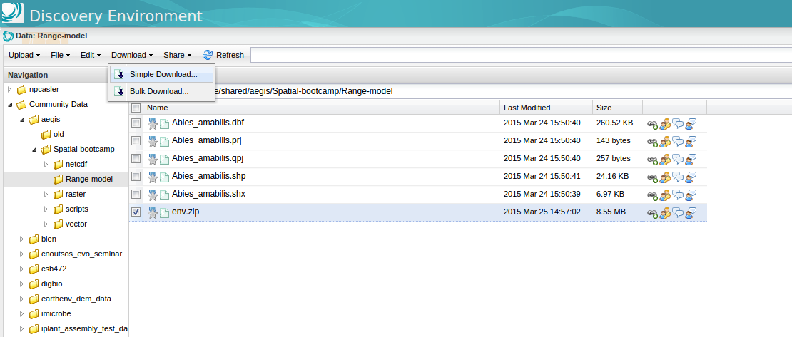
To download the layers, sign in to the iPlant Discovery Environment and open the Data Store.

The layers should be available under /iplant/home/shared/aegis/Spatial-bootcamp/Range-model/env.zip

To download the archive, check the file and click Download > Simple Download in the Menu bar.

Download the zip file to your workspace and unzip the directory. You should find a group of ascii rasters.

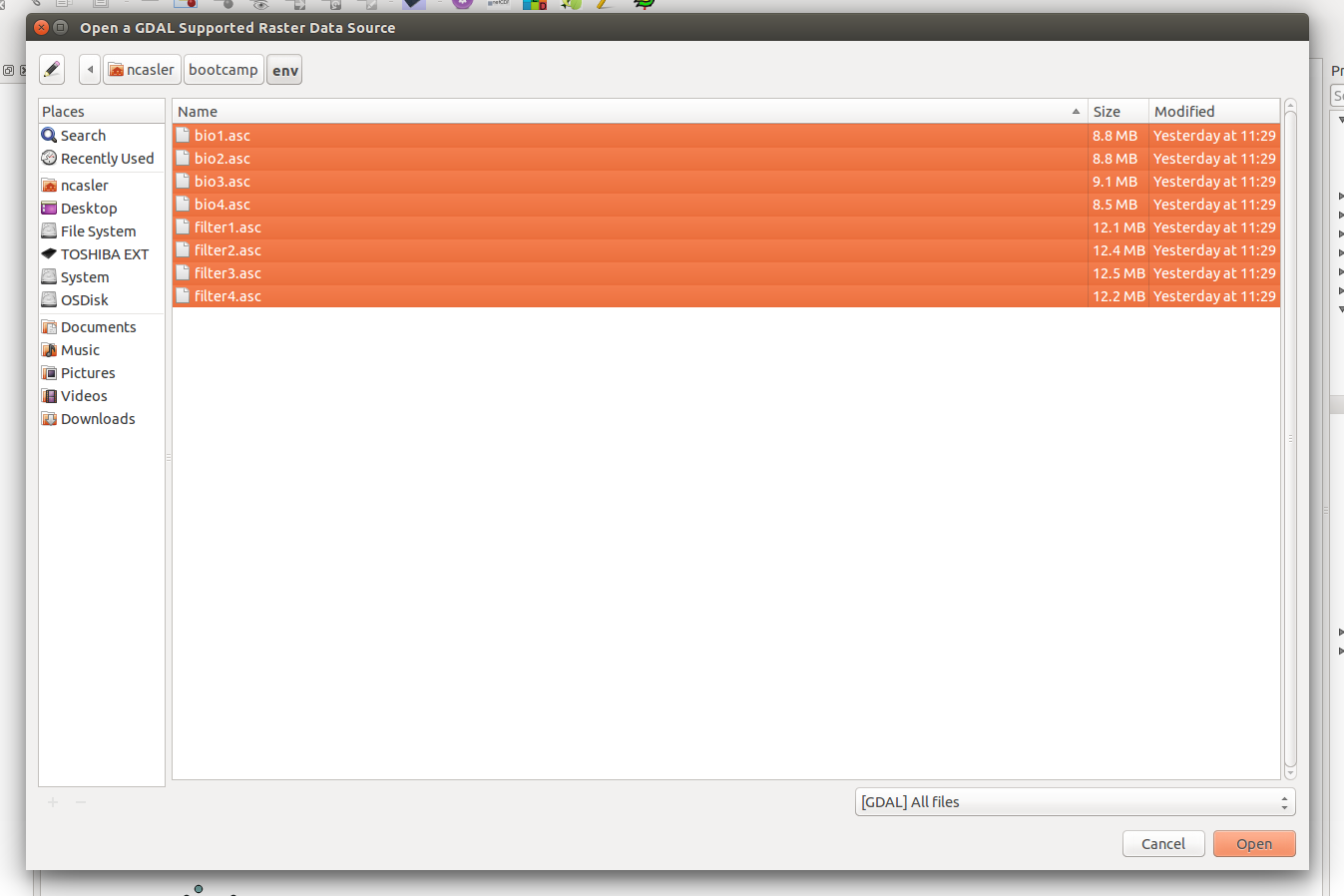
You can load the ascii rasters into QGIS as Raster datasets.

Click the Add Raster button, navigate to the unzipped directory and select all of the ascii rasters.

Once all the rasters are loaded, you should see them in your Table of Contents, but not on the map.

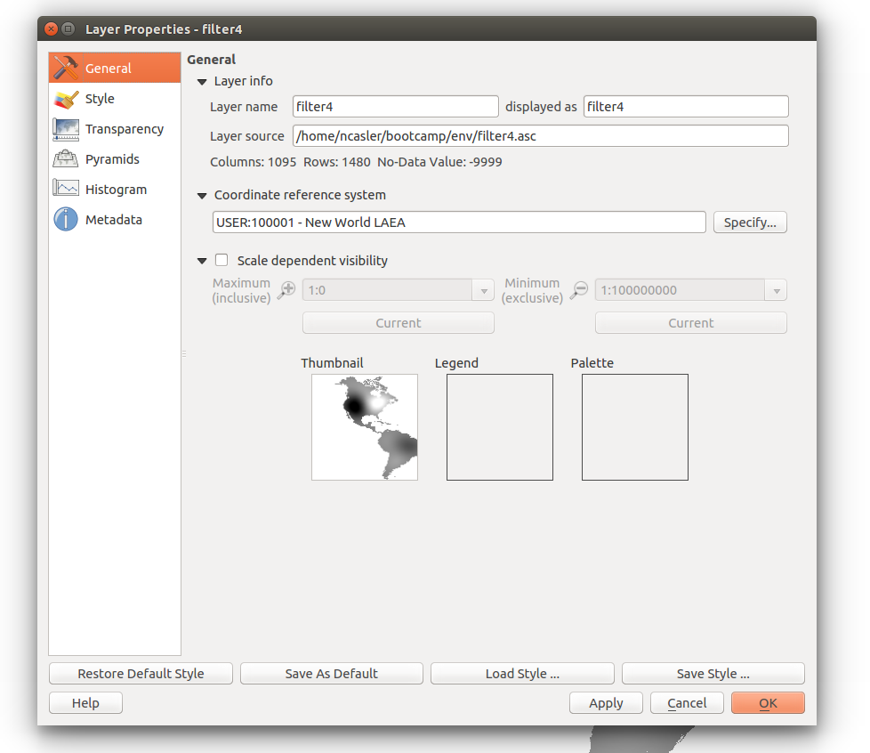
If you check the layer properties on one of the rasters, you can see that they default to EPSG:4326, although we had previously stated they come in the New World LAEA.

This happens because Ascii Grid Format doesn’t store any projection information.

To allow any analysis, we will have to define the projection for the raster data sets.

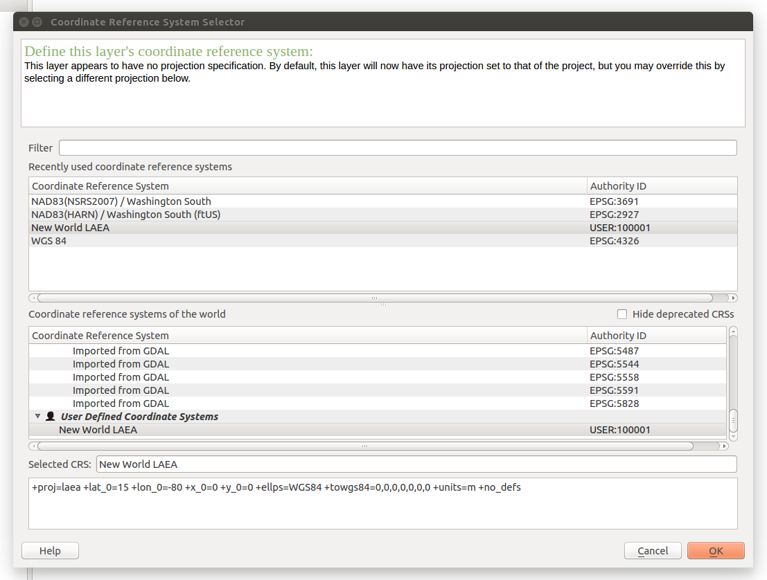
To do this, you can click on the layer name in the Table of Contents and Select Set Layer CRS

Select New WOrld LAEA from the list of projections and click OK

Check the layer properties to make sure the projection has been set.

Repeat the above steps for each of the ascii rasters until they all have the proper projection.

SWD creation

To create the SWD, we need to sample the environmental variable layers at the observation points. To do this, we will need to install the Point Sampling Plugin.

In the top menu, click Plugins > Manage and Install Plugins…

Click Get more in the left menu and Search for Point sampling

Click Install plugin and check that it is enabled under the list of installed plugins.

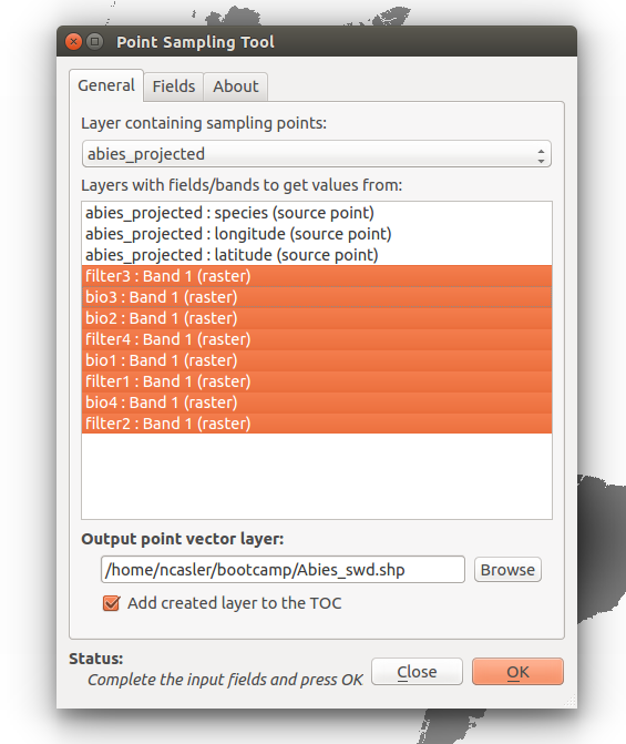
Navigate to Plugins > Analyses > Point Sampling Tool

In the dialog that opens, select abies_projected as the Layer containing sampling points

Under Layers with fields/bands to get values from: Select all of the environmental layers with type (raster)

Under Output point vector layer: Click Browse and select the location for the output.

Name the output Abies_swd.shp and make sure Add created layer to the TOC is checked

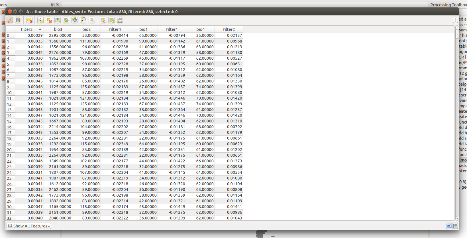
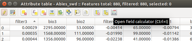
To make sure that the point sampling worked, we will check the new attribute table.

We are almost done with our SWD, the next step is to add a column with the species name.

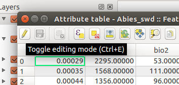
While we are in the attribute table you can add a column using the field calculator.

First, we need to Start an editing session on our attribute table by clicking the Toggle Edits Button in the upper left corner of the table.

Next, open the Raster Calculator on the right side of the toolbar.

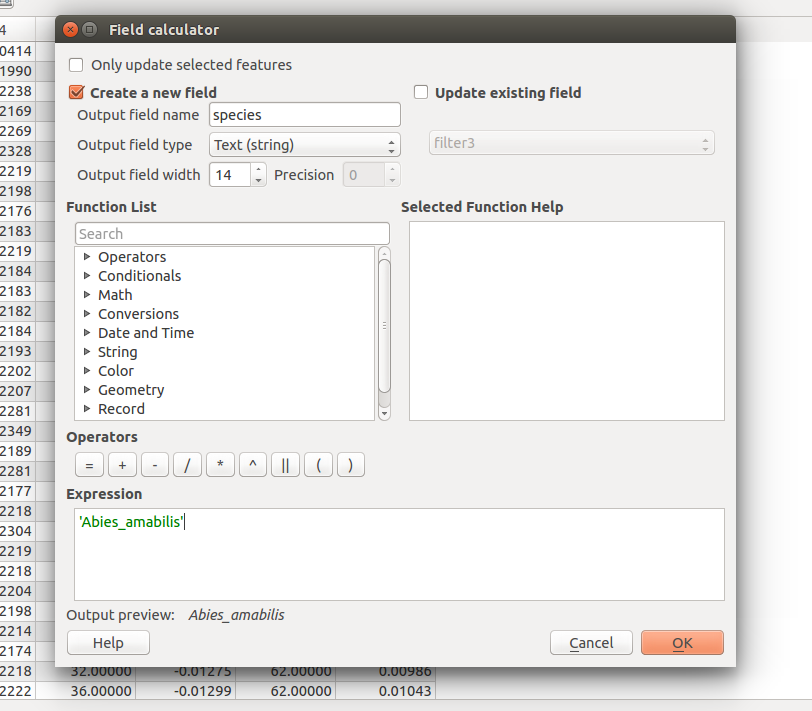
In the dialog that opens, make sure that *Create a new field is checked.

Set the output field name to species with a field type of Text (string) and a length of 14

Set the expression to ‘Abies_amabils’ to set the value for each row to the species name.

Once the column has been added, save your edits by hitting the Save Edits Button next to the Toggle Edits Button.

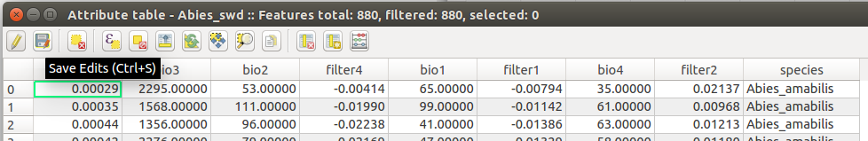
Now that we have our species name in the table, we need to create a csv for Maxent to read.