Landslide Susceptibility
Landslide Susceptibility Model
Overview
This case study has been chosen to demonstrate the concepts being highlighted by the bootcamp. We have chosen a landslide susceptibility analysis due to the diversity of inputs and a general curiousity into the methodology. The study area has been chosen in response to the Oso Mudslide1 which took place in Washington State on March 22nd, 2014. The methodology for this analysis is based off of work done by the California Geological Survey in Conjunction with the USGS2.
Project Definition
- Location: Washington State
- Bounding Coordinates: (-125.3424, 44.9408), (-115.8, 49.779)
- Resolution: 1 km
- Projection: Washington State Plane South (US ft) 3
- EPSG:2927
Data Collection
Data types: Landslides are discrete phenomena that should be represented using vector data, but are caused by a variety of continuous and discrete conditions so our inputs will include raster, and vector data sets.
| Input Layer | Data Source | |
|---|---|---|
| DEM | GTopo303 | |
| Geology | Washington Dept. of Natural Resources4 | |
| Landslide Inventory | Washington Dept. of Natural Resources4 | |
| Washington Boundary | Global Administrative Areas5 | |
| Daily Precipitation | Earth System Research Laboratory(NOAA)6 |
The DEM can be downloaded from ftp://edcftp.cr.usgs.gov/data/gtopo30/global/w140n90.tar.gz
This tarball can be extracted using an archive extraction application like 7-zip.
(Note: if you are using 7-zip or winRAR to extract the file, you will have to extract the .gz first. Then extract the .tar file from within the extracted subdirectory.)
If you are using Mac or Linux you can extract the files in the terminal with the following command:
tar -zxvf w140m90.tar.gzData Wrangling
- Set project projection to EPSG:2927
Before starting any project in a GIS program, you should first set the project projection to make sure your data comes in with the same extent.
If you don’t set the project’s projection, the program will use the projection of the first layer added or EPSG:4326.
You can set the projection with the following steps:
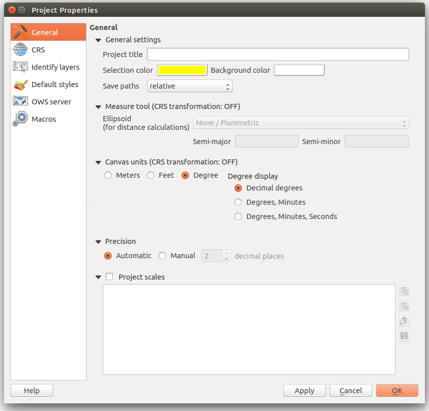
- In the top navbar go Project > Project Properties
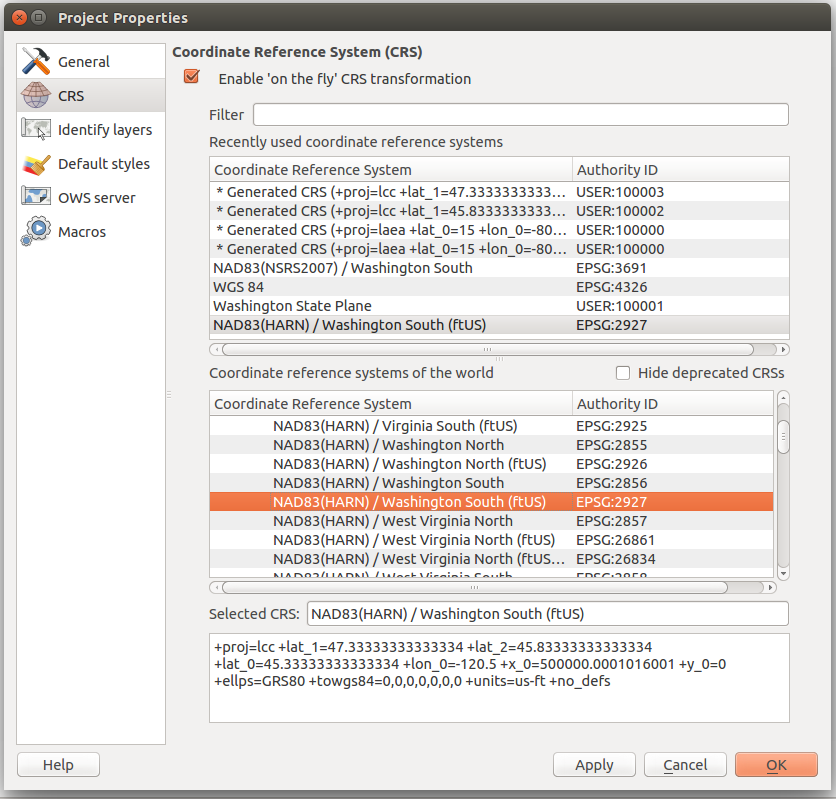
- Select CRS in the Left menu
- Check Enable On-the-fly CRS transformation
- Select NAD83(HARN)/Washington South(ftUS) EPSG:2927 from the List of Projections
- Add the US States shapefile
Since our project is directed at the state of Washington. We should extract the Washington state boundary for our study. The GADM6 project provides high-quality boundary data on country,state and county levels. We can use the US-state level dataset to get the Washington boundary.
- Select Add Vector Layer in the left toolbar
- Browse to the USA_adm1.shp layer from the iPlant Data Store
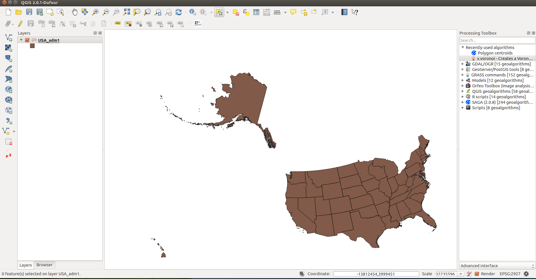
- Create a layer for the state of Washington
- In the top toolbar, select Select Single Feature
- Click on the state of Washington to select it
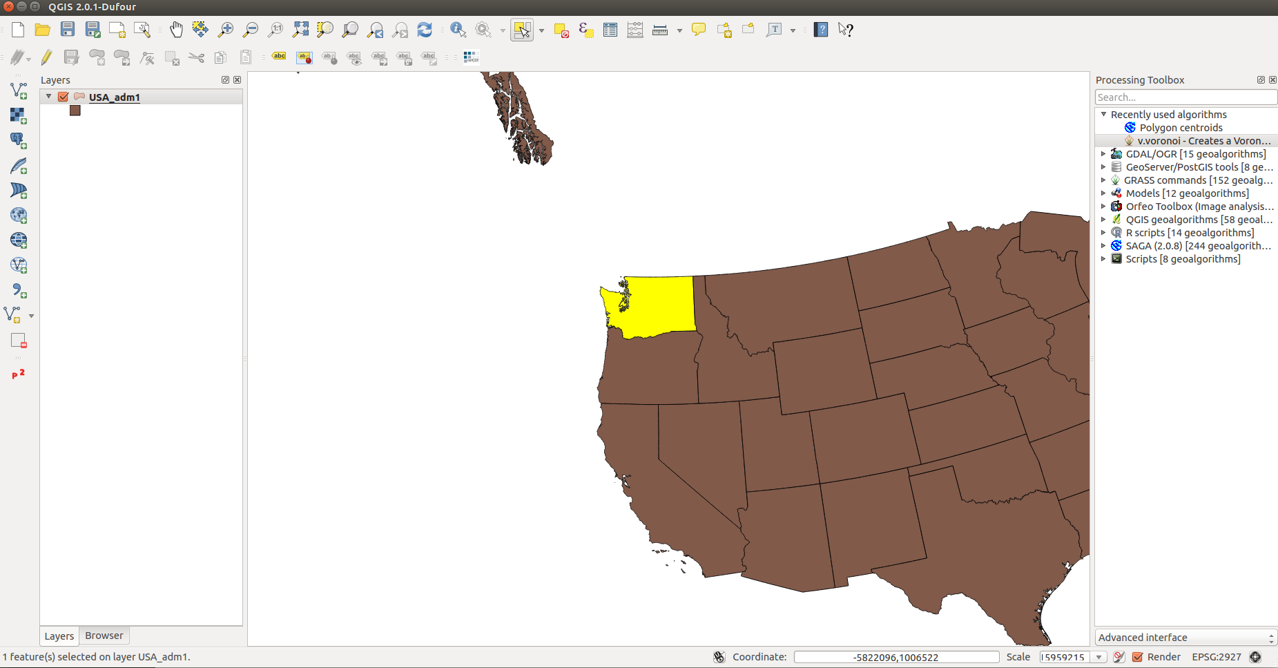
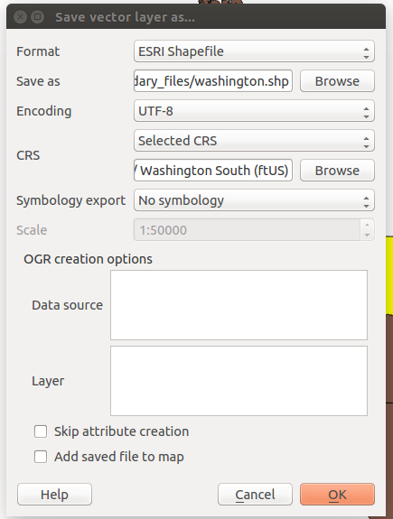
- Right click on the USA_adm1 layer and select Save Selection As…
- Format: ESRI Shapefile
- Save as: washington.shp
- Encoding: UTF-8
- CRS:
- Project CRS
- Browse > NAD83(HARN)/Washington South (ftUS) EPSG:2927
- Load the new washington layer
- Select Add Vector Layer
- Browse to the new washington layer and click Open
- Remove the USA_adm1 layer from the project
Now that we have the Washington layer, we can get rid of the U.S. layer.
- Right click the layer in the table of contents
- Select Remove
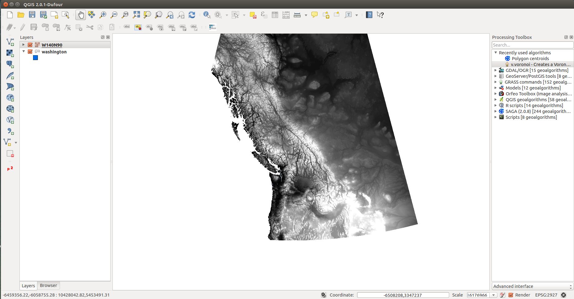
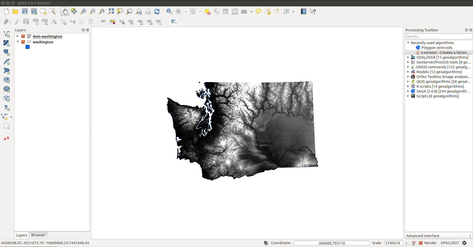
- Add the DEM layer from the iPlant data store
DEMs or Digital Elevation Models are very useful for establishing topological context in a map. DEMs generally come as a raster dataset that consists of elevation values. There are several different byproducts that can be created from DEMs.
This DEM was taken from the GTOPO30 satellite data.
- In the left toolbar, select Add Raster Layer
- Select source_files/W140N90.DEM
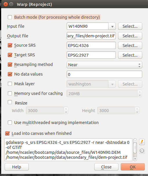
- Project the dem to EPSG:2927
- In the top menu, go to Raster > Projections > Warp (Reproject)
- Use the following options
- Input File: W140N90
- Output File: secondary_files/dem-project.tif
- Source SRS: EPSG:4326
- Resampling Method: Near
- No data values: 0
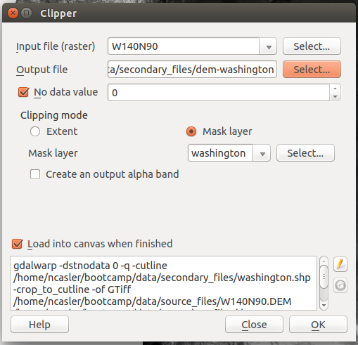
- Clip the dem to the shapefile
- In the top menu, select Raster > Extraction > Clipper
- In the window, set the following options:
- Input file: dem-project.tif
- Output file: dem-washington.tif
- No data value: 0
- Clipping Mode: Mask layer > washington
- Load into canvas when finished
- Remove the W140N90 layer
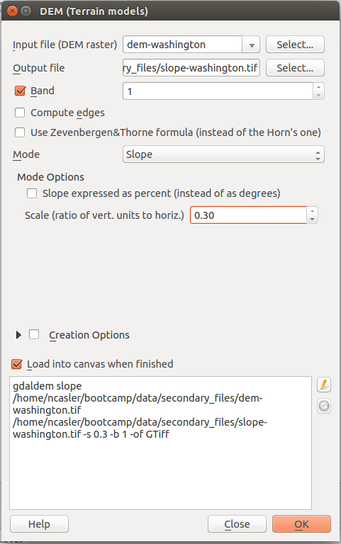
- Create a slope surface
In the top menu, select Raster > Analysis > DEM
- Input file: dem-washington
- Output file: slope-washington.tif
- Mode: Slope
- Scale: 0.30
- Load into canvas when finished
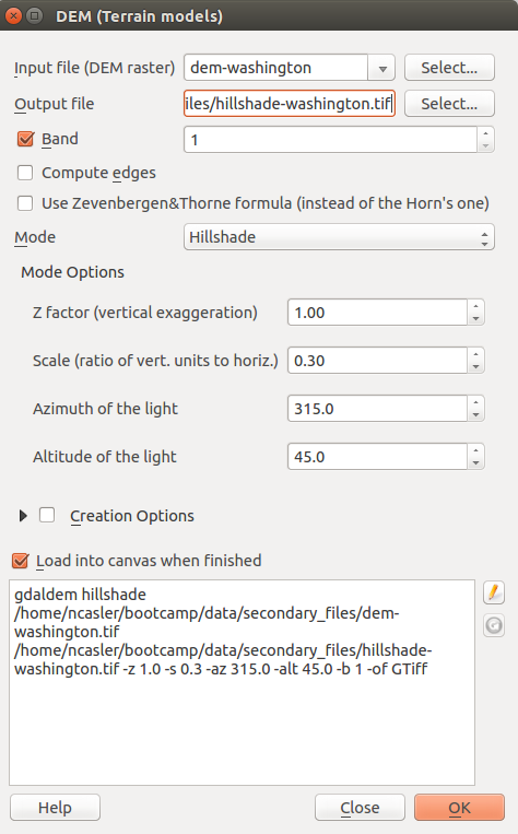
- Create a hillshade layer
In the top menu, select Raster > Analysis > DEM
- Input file: dem-washington
- Output file: hillshade-washington.tif
- Mode: Hillshade
- Z factor: 1.0
- Scale: 0.30
- Azimuth of light: 315.0
- Altitude of light: 45.0
- Load into canvas when finished
Data Analysis
i Reclassifying inputs:
Slope
| Category | Slope | |
|---|---|---|
| 1 | < 3° | |
| 2 | 3-5° | |
| 3 | 5-10° | |
| 4 | 10-15° | |
| 5 | 15-20° | |
| 6 | 20-30° | |
| 7 | 30-40° | |
| 8 | > 40° |
In order to reclass our slope layer into something useful, we will use the grass r.reclass tool
The r.reclass tool reads text files which define the classification rules(rule files). For this example, our rule fill will have the following contents:
slope-rule.txt
0 thru 2.99 = 1
3 thru 4.99 = 2
5 thru 9.99 = 3
10 thru 14.99 = 4
15 thru 19.99 = 5
20 thru 29.99 = 6
30 thru 39.99 = 7
40 thru 90 = 8
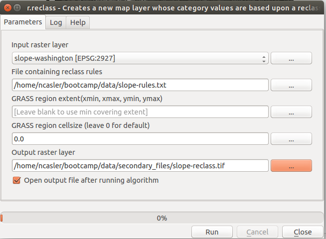
Once we have created the slope rule file. We can select the r.reclass tool from the Processing Toolbox.
In the processing toolbox, select GRASS commands > Raster > r.reclass
We will use the following settings for the reclassify tool:
- Input Raster: slope-washington
- File containing reclass rules: slope-rules.txt
- Output raster layer: slope-reclass.tif (NOTE: select Save to file… or else QGIS will not create a permanent output)
Susceptibility
We will have to do some raster calculations to create the output data set. The classifications are taken from the California study2 and are as follows:
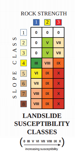
Since we need to cross reference these categories, we need to create a raster which represents each unique combination of the slope and rock strength classes. A method to create unique combinations is to promote the rock strength categories a decimal place. This would make the rock classes: 10,20, and 30.
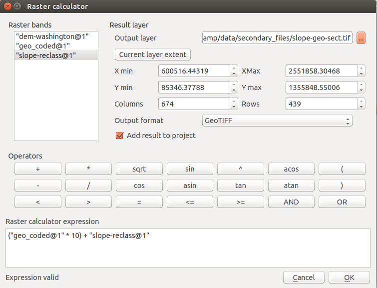
To create these new classes, we can load the source_files/geo_coded.tif, and secondary_files/slope_reclass.tif
In the top menu, select Raster > Raster Calculator
Our raster calculator expression will be:
("geo_coded@1" * 10) + "slope-reclass@1"Output layer: slope-geo-sect.tif
We can apply the landslide susceptibility classification using r.reclass and the following rule file:
landslide-rule.txt
11 12 13 21 31 = 0
14 = 3
22 23 = 5
15 = 6
16 32 33 = 7
17 18 24 = 8
25 thru 28 34 = 9
35 thru 38 = 10
Precipitation
Now that we have created the landslide susceptibility layer, we can make use the Average Annual Precipitation layer to check the susceptible areas against the areas receiving the most annual rain.
Convert millimeters to inches
Raster calculator: precip = precip * 0.0394
Check THIS STEP AGAINST REFERENCES
| Category | Precipitation | |
|---|---|---|
| 0 | ||
| 1 | 5-10 in | |
| 2 | 10-15 in | |
| 3 | 15-30 in | |
| 4 | 30-45 in | |
| 5 | 45-60 in | |
| 6 | 60-75 in | |
| 7 | 75-90 in | |
| 8 | > 90 in |
Visualization
Now that the output datasets have been created, we can work on making our results presentable.
Go to Cartography & Visualization…
-
http://www.usgs.gov/blogs/features/usgs_top_story/landslide-in-washington-state ↩
-
http://www.conservation.ca.gov/cgs/information/publications/Documents/MS58.pdf ↩ ↩2
-
http://www.dnr.wa.gov/ResearchScience/Topics/GeosciencesData/Pages/gis_data.aspx ↩ ↩2
-
http://gadm.org/country ↩
-
http://www.esrl.noaa.gov/thredds/catalog/Datasets/cpc_us_precip/catalog.xml#Datasets/cpc_us_precip/RT ↩ ↩2